Plot Audio Spectrogram

In this example we will plot the audio spectrogram using RedPandas. The steps are very similar to the previous example where we plotted the audio waveforms.

Running the example

The first step is to load RedVox data into a DataWindow.

from redvox.common.data_window import DataWindow

# Input Directory
input_dir = "path/to/redvox/data/dw_1648830257000498_2.pkl.lz4"

# Load data window from report
dw = DataWindow.deserialize(input_dir)

The next step is to make a pandas dataframe using RedPandas redpd_dataframe.

from redvox.common.data_window import DataWindow
from redpandas.redpd_df import redpd_dataframe

# Input Directory
input_dir = "path/to/redvox/data/dw_1648830257000498_2.pkl.lz4"

# Load data window from report
dw = DataWindow.deserialize(input_dir)

# Make a pandas DataFrame, where crucial information from DataWindow is extracted
# In this case, we are only extracting 'audio' from the DataWindow but other sensors such as 'barometer',
# 'accelerometer', 'gyroscope', 'magnetometer', 'health', or 'location' are possible
rp_df = redpd_dataframe(input_dw=dw,
                        sensor_labels=['audio'])

Calculate the Short-term Fourier transform using tfr_bits_panda.

from redvox.common.data_window import DataWindow
from redpandas.redpd_df import redpd_dataframe
from redpandas.redpd_tfr import tfr_bits_panda

# Input Directory
input_dir = "path/to/redvox/data/dw_1648830257000498_2.pkl.lz4"

# Load data window from report
dw = DataWindow.deserialize(input_dir)

# Make a pandas DataFrame, where crucial information from DataWindow is extracted
# In this case, we are only extracting 'audio' from the DataWindow but other sensors such as 'barometer',
# 'accelerometer', 'gyroscope', 'magnetometer', 'health', or 'location' are possible
rp_df = redpd_dataframe(input_dw=dw,
                        sensor_labels=['audio'])

# Calculate time frequency representation (TFR)
tfr_bits_panda(df=rp_df,  # the name of the redpandas dataframe, in this case rp_df
               sig_wf_label="audio_wf",  # Column label with sensor data, in this case audio
               sig_sample_rate_label="audio_sample_rate_nominal_hz",  # Column label with sample rate
               order_number_input=12,  # Optional, default=3
               tfr_type="stft")  # Optional, 'stft' or 'cwt, default='stft'

# tfr_bits_panda will make 3 new columns with the time frequency representation: 'tfr_bits', 'tfr_time_s',
# 'tfr_frequency_hz'. Double check they are strored in the dataframe
print(f'Check for "tfr_bits", "tfr_time_s", "tfr_frequency_hz":\n{rp_df.columns.values}')

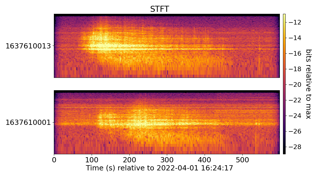
Let’s plot the spectrogram with plot_mesh_pandas .

from redvox.common.data_window import DataWindow
from redpandas.redpd_df import redpd_dataframe
from redpandas.redpd_tfr import tfr_bits_panda
from redpandas.redpd_plot.mesh import plot_mesh_pandas
import matplotlib.pyplot as plt

# Input Directory
input_dir = "path/to/redvox/data/dw_1648830257000498_2.pkl.lz4"

# Load data window from report
dw = DataWindow.deserialize(input_dir)

# Make a pandas DataFrame, where crucial information from DataWindow is extracted
# In this case, we are only extracting 'audio' from the DataWindow but other sensors such as 'barometer',
# 'accelerometer', 'gyroscope', 'magnetometer', 'health', or 'location' are possible
rp_df = redpd_dataframe(input_dw=dw,
                        sensor_labels=['audio'])

# Calculate time frequency representation (TFR)
tfr_bits_panda(df=rp_df,  # the name of the redpandas dataframe, in this case rp_df
               sig_wf_label="audio_wf",  # Column label with sensor data, in this case audio
               sig_sample_rate_label="audio_sample_rate_nominal_hz",  # Column label with sample rate
               order_number_input=12,  # Optional, default=3
               tfr_type="stft")  # Optional, 'stft' or 'cwt, default='stft'

# tfr_bits_panda will make 3 new columns with the time frequency representation: 'tfr_bits', 'tfr_time_s',
# 'tfr_frequency_hz'. Double check they are strored in the dataframe
print(f'Check for "tfr_bits", "tfr_time_s", "tfr_frequency_hz":\n{rp_df.columns.values}')

# Plot spectrogram
plot_mesh_pandas(df=rp_df,
                 mesh_time_label="tfr_time_s",  # Column label for TFR timestamps
                 mesh_frequency_label="tfr_frequency_hz",   # Column label for TFR frequency
                 mesh_tfr_label="tfr_bits",  # Column label for TFR bits
                 t0_sig_epoch_s=rp_df["audio_epoch_s"][0][0],  # The first timestamp
                 sig_id_label="station_id",  # Column name with IDs/names of stations, important for y ticks
                 frequency_hz_ymin=1.,
                 frequency_hz_ymax=200.,
                 frequency_scaling='log',
                 ytick_values_show=True,  # show y ticks for frequency
                 common_colorbar=True,  # add colorbar
                 )

plt.show()

Example output

Running the above code snippet should yield the following figure:

You can also view this example in Github.