Load the Accelerometer Data

In the previous example, we loaded single-channel audio data. The next step is to load three-channel data from the accelerometer (X, Y and Z dimensions) following a similar process as the audio data.

Running the example

The first step is to load RedVox data in a DataWindow.

from redvox.common.data_window import DataWindow

# Input Directory
input_dir = "path/to/redvox/data/dw_1648830257000498_2.pkl.lz4"

# Load data window from report
dw = DataWindow.deserialize(input_dir)

Next, extract the accelerometer data for each Station stored in the DataWindow.

from redvox.common.data_window import DataWindow

# Input Directory
input_dir = "path/to/redvox/data/dw_1648830257000498_2.pkl.lz4"

# Load data window from report
dw = DataWindow.deserialize(input_dir)

# Loop to extract accelerometer data from all stations
for station in dw.stations():
    # Check that there is accelerometer data in the first place
    if station.has_accelerometer_data():
        # Accelerometer has 3 channels - x, y and z
        accelerometer_x_samples = station.accelerometer_sensor().get_accelerometer_x_data()
        accelerometer_y_samples = station.accelerometer_sensor().get_accelerometer_y_data()
        accelerometer_z_samples = station.accelerometer_sensor().get_accelerometer_z_data()
        # The channels share the same timestamps - format to seconds
        accelerometer_time_micros = station.accelerometer_sensor().data_timestamps() - station.accelerometer_sensor().first_data_timestamp()
        accelerometer_time_s = accelerometer_time_micros*1E-6

We can plot the accelerometer data using the Matplotlib library to visualize it.

from redvox.common.data_window import DataWindow
import matplotlib.pyplot as plt

# Input Directory
input_dir = "path/to/redvox/data/dw_1648830257000498_2.pkl.lz4"

# Load data window from report
dw = DataWindow.deserialize(input_dir)

for station in dw.stations():
    # Check that there is accelerometer data in the first place
    if station.has_accelerometer_data():
        # Accelerometer has 3 channels - x, y and z
        accelerometer_x_samples = station.accelerometer_sensor().get_accelerometer_x_data()
        accelerometer_y_samples = station.accelerometer_sensor().get_accelerometer_y_data()
        accelerometer_z_samples = station.accelerometer_sensor().get_accelerometer_z_data()
        # The channels share the same timestamps - format to seconds
        accelerometer_time_micros = station.accelerometer_sensor().data_timestamps() - station.accelerometer_sensor().first_data_timestamp()
        accelerometer_time_s = accelerometer_time_micros*1E-6

        # Plot the acceleration data - one subplot per channel
        fig, ax = plt.subplots(nrows=3, ncols=1, sharex='col')
        ax[0].plot(accelerometer_time_s, accelerometer_x_samples)
        ax[1].plot(accelerometer_time_s, accelerometer_y_samples)
        ax[2].plot(accelerometer_time_s, accelerometer_z_samples)
    
        # Set labels and subplot title
        ax[0].set_ylabel(r'Acc X [$m/s^2$]')
        ax[1].set_ylabel(r'Acc Y [$m/s^2$]')
        ax[2].set_ylabel(r'Acc Z [$m/s^2$]')
        ax[2].set_xlabel(f"Seconds from {int(dw.start_date()*1E-6)} Unix epoch UTC")
    
        plt.suptitle(f"RedVox Station ID {station.id()}")

plt.show()

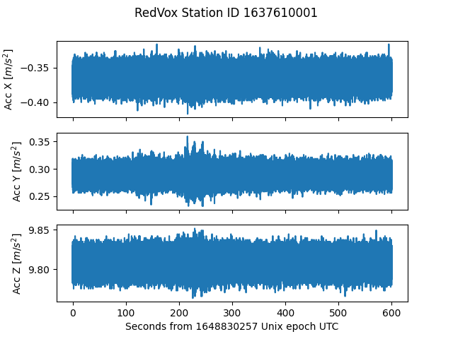
Example output

After running the above code snippet, the following graph should appear:

For a more complete example on how to load accelerometer sensor data, visit Github.

In the next section, we will take a look at loading other sensors such as the barometer and the magnetometer.